(Solution) TL2LOM – Logistics Modelling Assignment
Solution
Transport Optimization for a Logistics Firm
Introduction
Transportation cost is a major component of total logistics expenditure and a frequent target for operational optimization in logistics firms. Linear programming (LP) provides a framework from which one can be able to pick and decide the optimal mix of resources. Under the LP model, costs are assumed to be linear allowing one to express variable as linear functions (Hillier & Lieberman, 2024). Our key objective in this report is to use two variables to formulate a transport optimization model. We will use the LP model to find the minimal costs of running the model and put the test results through sensitivity analysis and managerial discussion.
Model assumptions
The LP model seeks to minimize weekly transportation costs based on two trucks with different capacities, operational costs and constraints (Chopra, 2025). The logistics firm transports goods weekly between a central warehouse and a regional distribution hub. The firm operates two trucks: Truck 1 has 10-tonne capacity and Truck 2 has 15-tonne capacity. The logistics firm is meant to transport at least 300 tonnes weekly. The firm is using the LP model to determine the number of weekly departures for each truck that minimizes operational cost while satisfying constraints imposed by driver hours, maintenance schedules, and operating budgets.
Let denote the number of weekly departures using Truck 1, which is a smaller truck. Let denote the number of weekly departures using Truck 2. Both and are continuous and non-negative. The total operating cost per departure for Truck 1 is $500, and for Truck 2 is $650. The objective function is therefore to minimize total weekly cost expressed as:
Constraints
The model will include the following six constraints (Taha, 2019) i.e.
- The two trucks must meet the demand of at least 300 tonnes per week, with Truck 1 carrying 10 tonnes per departure and Truck 2 carrying 15 tonnes:
- We have a labor constraint of at most 300 driver-hours per week, with the departure of Truck 1 consuming 8 driver-hours and Truck 2 consuming 10 driver-hours; the fleet’s drivers supply:
- Maintenance and scheduling limit Truck 1 departures to at most 20 per week:
- Truck 2 departures are limited to at most 18 per week:
- We have a weekly operational budget constraint of 20,000 thus the total amount of the departures is:
- Nonnegativity:
The LP formulations used above in our model are also widely used approaches in transport and supply chain optimization (Chopra, 2025).
Graphical representation
To get the point of intersection of each of the assumption parameters, we need to compute and plot the area of each line and draw the lines, i.e.,
- Demand line: .
- Driver-hours line: .
- Vertical line: .
- Horizontal line: .
- Budget line: .
| Equations | (x, y) axis plots | ||||
| (3,18) | (5,16.667) | (6,16) | (9,14) | (10,13.33) | |
| (3,27.6) | (5,26) | (6,25.2) | (9,22.8) | (10,22) | |
| (20,3) | (20,5) | (20,6) | (20,9) | (20,10) | |
| (3,18) | (5,18) | (6,18) | (9,18) | (10,18) | |
| (3,77.6) | (5,76) | (6,75.2) | (9,72.8) | (10,72) | |
The different lines produce the graphs below, plotted as an image. Where the various graphs intersect at the feasible region. The feasible region is the set of that satisfy all five inequalities simultaneously. Winston, (2008)
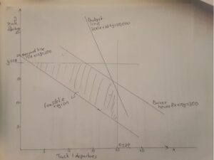
The feasible region is the set of that satisfy all five inequalities simultaneously. Winston, (2008) states that to get the feasible region, one should check the point of intersection and look for the optimal area that reduces every inequality.
The point of intersections between the constraints are at the below points:
- , the intersection of with the demand line, i.e. .
- , the intersection of the demand line with .
- , the intersection of with the driver-hours line .
- , the intersection of the driver-hours line with .
Each of these points is an intersection between two points. According to LP theory, the optimal value is the minimum value of the intersection, considering the objective is linear and the feasible set is convex (Hillier & Lieberman, 2024).
Evaluating the objective function at the candidate corners yields the following weekly costs:
- At : .
- At : .
- At : .
- At : .
Therefore, the minimum occurs at with weekly cost $13,200. This solution meets the demand exactly (capacity used equals 300 tonnes because ), and it uses the maximally allowed Truck 2 departures. There is capacity remaining within the driver-hours and budget constraints at this capacity, while the demand constraint and the Truck 2 maximum constraint are binding.